The State Monad Math and programming stuff
Merge Sort

Lion tamer illustration by Jason Holley
Merge sort is a pretty efficient comparison-based sorting algorithm; It’s a divide and conquer algorithm that was invented by John von Neumann in 1945.
Conceptually, merge sort is actaully a pretty simple algorithm:
-
Divide the unsorted list into n sublists, each containing one element (this is the base case; a list of one element is considered sorted).
-
Merge these sublists to produce new sorted sublists until there is only one sublist remaining.

A more hands on explanation of the algorithm can easily be found pretty much anywhere on the internet. This video by GeeksforGeeks does a pretty good job at explaining the algorithm with some nice animations.
Today we will be answering one question. Why does merge sort run in $\mathcal{O}(n\space log(n))$ (Worst-case performance).
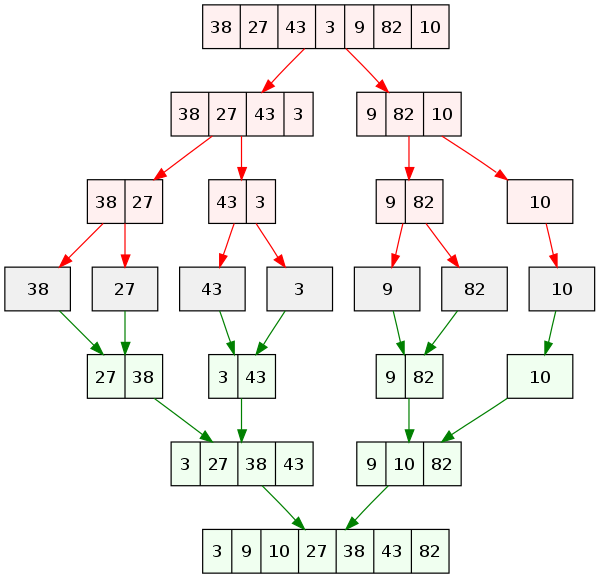
It is easily seen from the previous diagram that the algorithm splits up the problem of sorting an array of $n$ elements into a tree with $n$ leaves. In each level of said tree some certain amount of work is performed. In order to understand how merge sort works and why it takes precisely $n\space log(n)$ in the worst case we must first find out know how much work is performed on each level of the binary tree.
So basically, our algorithm does two things:
splitting and merging.
Let’s analyze the merging subroutine first:
What is the worst case comparisons?
Example:
Let a1 and a2 be two sorted sub-arrays of length n = 3 each. How many comparisons do we need in order to merge them into one sorted array of length N=6?
- a1 = (1, 2, 3)
- a2 = (-1, 0, 6)
We will put a pointer at the first element of each list.
- a1 = ( –> 1, 2, 3)
- a2 = ( –> -1, 0, 6)
We compare 1 and -1. The lesser item (-1) wins and gets to take its place on the sorted array:
sortedArray = ( -1 _ _ _ _ _ )
(1 comparison)
We move the pointer of a2 forward:
- a1 = ( –> 1, 2, 3)
- a2 = (-1, –> 0, 6)
We compare 1 and 0. The lesser item (0) wins.
sortedArray = ( -1 0 _ _ _ _ )
(2 comparison)
We move the pointer of a2 forward:
- a1 = ( –> 1, 2, 3)
- a2 = (-1, 0, –> 6)
We compare 1 and 6. The lesser item (1) wins.
sortedArray = ( -1 0 1 _ _ _ )
(3 comparison)
We move the pointer of a1 forward:
- a1 = (1, –> 2, 3)
- a2 = (-1, 0, –> 6)
We compare 2 and 6. The lesser item (2) wins.
sortedArray = ( -1 0 1 2 _ _ )
(4 comparison)
We move the pointer of a1 forward:
- a1 = (1, 2, –> 3)
- a2 = (-1, 0, –> 6)
We compare 3 and 6. The lesser item (3) wins.
sortedArray = ( -1 0 1 2 3 _ )
(5 comparison)
Since we can’t move the pointer of a1 anymore and the only element left in a2 is 6 we simply put 6 at the end of the sorted array.
sortedArray = ( -1 0 1 2 3 6 )
And this is our final sorted array.
mergesort used $5 = n-1$ comparisons to merge two sorted sub-arrays. The is the worst case comparisons for the merge subroutine. $\mathcal{O}(n)$
Now that we know the time complexity for the merge subroutine we can finally tackle the big boy merge sort.
Let $T(n)$ denote the time running time of merge sort. Then, it is easy to see that the following equality is true:
\[T(n)=T\left(\frac{n}{2}\right)+T\left(\frac{n}{2}\right)+(n-1),\]where we have split the total work into two subroutines $T\left(\frac{n}{2}\right)$ plus the merging operation.
We can perform this spitting once more:
\[T(n)= T\left(\frac{n}{4}\right) + T\left(\frac{n}{4}\right) + T\left(\frac{n}{4}\right) + T\left(\frac{n}{4}\right) + \left(\frac{n}{2}-1\right) + \left(\frac{n}{2}-1\right) + (n-1)\] \[T(n)=4T\left(\frac{n}{4}\right)+2\left(\frac{n}{2}-1\right)+(n-1)\]We can go on forever…. Let us consider the case $n=8$.
\[T(8)=2T\left(\frac{8}{2}\right)+(8-1)\] \[T(8)=2T\left(4\right)+(7)\]Applying our recursive definition…
\[T(8)=2T\left(2\right)+2T\left(2\right)+2(3)+(7)\] \[T(8)=2T\left(1\right)+2T\left(1\right)+2T\left(1\right)+2T\left(1\right)+4(1)+2(3)+(7)\]But since we know that $T(1)=0$, that is for an array of one element we don’t need to compare anything.
\[0+0+0+0+4+6+7=17\]17 total comparisons.
It’s important to notice that no actual work is done until the last bit of the algorithm when the merging is performed, in other words, the splitting part of the algorithm doesn’t do any comparisons.
The General Case
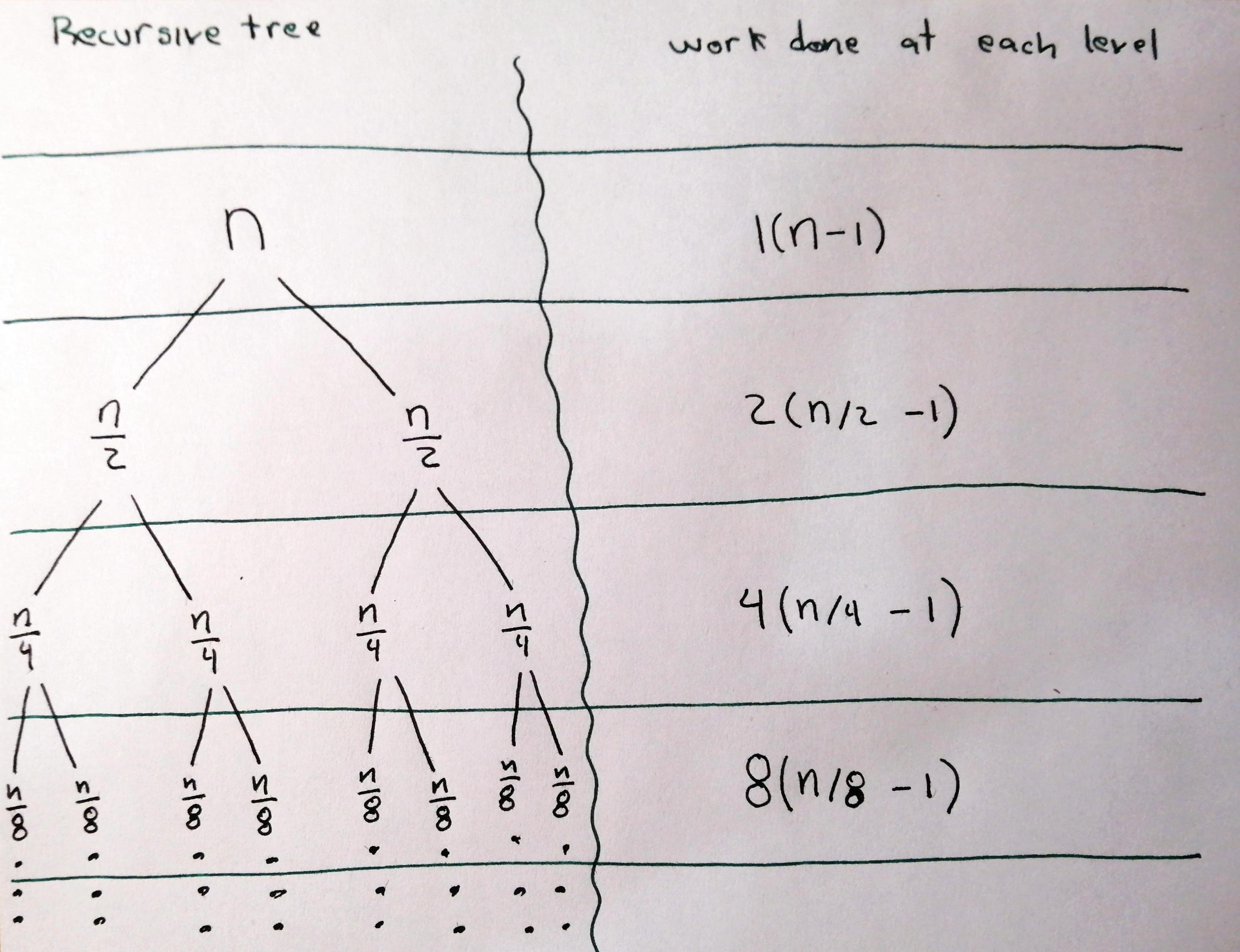
From the previous example we know that the only significant work that is done on each level is merging. We can see this in the following diagram:

There is a pattern emerging…
In general, the work performed on the $i^{th}$ level is $2^{i}\left(n/2^i-1\right)$
We can sum the work done on each level to find out the total work:
But how many levels are there? Well, since we are splitting our array into 2 sub-arrays and then splitting those 2 sub-arrays into another 4 sub-arrays and so on we know that our tree will have exactly $log_{\space 2}(n)$ levels. In fact, the height of a binary tree is always $\mathcal{O}(log(n))$
\[\sum^{log(n)-1}_{0}2^{i}\left(n/2^i-1\right)= \sum^{log(n)-1}_{0}\left(n-2^{i}\right)= \sum^{log(n)-1}_{0}n-\sum^{log(n)-1}_{0}2^{i}\]Notice we’re summing from 0 to $log(n)-1$ and not $log(n)$. This is because indexing in most programming languages start from zero. This way we sum from level zero to level $(n-1)$ where $n$ is the length of our array.
\[\left[\left(log(n)-1-0\right)-1\right]n-(1+2+4+\dots 2^{log(n)-1})\] \[n\space log(n)-\frac{(2)^{(log(n)-1)+1}-1}{(2)-1}\] \[n\space log(n)-(2)^{log(n)}-1\] \[n\space log(n)-(n-1)\] \[n\space log(n)-n+1\]The leading term in this expression is $n\space log(b)$, therefore our worst time running time is $\mathcal{O}(n\space log(n))$.
$\square$
Furthermore, merge sort uses extra space proportional to $n$.
This follows directly from the fact that the auxiliary array needed in merge needs to be of size at least $n$ for the last merge.
This completes a basic analysis of merge sort.
Written on January 16th, 2021 by José María Landa Chávez